Chebyshev's Inequality Calculator
Find the minimum proportion of any dataset that falls within k standard deviations of the mean, and the maximum that can fall outside, using Chebyshev's inequality. Type k directly, or derive it from a mean, standard deviation, and a range. Works for any distribution.
This is a distribution-free lower bound, not the exact proportion of your data within k standard deviations. It guarantees a worst-case minimum that holds for every distribution; for bell-shaped data the true figure is usually much higher.
Chebyshev bound
At least this much data within k SDs 75.00%
- Effective k used
- 2
- Minimum proportion within k SDs
- 0.7500
- At most this much data outside k SDs
- 25.00%
- Maximum proportion outside k SDs
- 0.2500
- Guaranteed minimum count within k SDs (of n)
- 75
- Within k SDs (guaranteed minimum) 0.7500 75%
- Outside k SDs (maximum) 0.2500 25%
How k changes the guaranteed minimum
| k (standard deviations) | At least this much within k SDs |
|---|---|
| 1.5 | 55.56% |
| 2 | 75.00% |
| 2.5 | 84.00% |
How to use this calculator
- Pick how to set k. Choose direct to type k yourself, or interval to work it out from a mean, a standard deviation, and a range.
- In direct mode, enter k, the number of standard deviations from the mean. It has to be greater than 1.
- In interval mode, enter the mean, the standard deviation, and the lower and upper bounds. The tool finds the effective k from the nearer end of the range: it takes the smaller of two distances, the mean minus the lower bound and the upper bound minus the mean, then divides by the standard deviation.
- Add a sample size n if you have one. The tool then turns the proportion into a guaranteed minimum count of points within k standard deviations.
- Read your results: the minimum proportion within k standard deviations, the maximum proportion outside, each as a decimal and a percent, plus the guaranteed minimum count.
How it works
Chebyshev’s inequality, also called Chebyshev’s theorem, works for any dataset that has a finite mean and standard deviation, no matter its shape. It says at least 1 minus 1 over k squared of the values sit within k standard deviations of the mean, and at most 1 over k squared sit outside (Emory University Math Center; Wikipedia). Here k is how many standard deviations away from the mean you are measuring. The two parts always add up to all of your data.
You pick one of two modes. In direct mode you type k, and it has to be greater than 1. In interval mode you enter a mean, a standard deviation, and a range, and the tool back-solves the effective k for you. Only one mode is active at a time, so the inputs and the derived k for the other mode stay hidden.
At k of 2 the guarantee is at least 75 percent within and at most 25 percent outside. At k of 3 it rises to at least 88.89 percent within. k is the one lever that moves the answer: raise k and the guaranteed minimum within goes up, lower it and the minimum goes down.
Interval mode needs a valid setup. The standard deviation must be above 0, the lower bound must sit below the upper bound, and the mean must fall between them. If the derived k comes out at 1 or less, the bound says nothing, so the tool shows a status message instead of a misleading number.
Because the rule assumes nothing about the shape of your data, the bound is deliberately conservative. Real bell-shaped data usually has far more inside the interval than Chebyshev guarantees. The same generality makes it useful when no distribution can be assumed: NIST researchers used Chebyshev’s inequality to set a minimum sample size for evaluating fingerprint data (NIST).
Examples
These cases match what the calculator returns, so you can check your own setup.
If you choose direct mode with k of 2 and a sample size of 100, the tool returns an effective k of 2, at least 75 percent within 2 standard deviations, at most 25 percent outside, and a guaranteed minimum of 75 of your 100 points inside. The math is 1 over 2 squared, which is 0.25, so the minimum within is 1 minus 0.25.
If you raise k to 3 with the same 100 points, the guarantee tightens to at least 88.89 percent within and at most 11.11 percent outside, a floor of 88 points inside. Here 1 over 3 squared is about 0.1111, and the count floors 88.8889 down to 88.
If you switch to interval mode with a mean of 70, a standard deviation of 5, a range from 60 to 80, and 200 points, the tool reads both distances as 10, divides by 5, and derives an effective k of 2. That again gives at least 75 percent within and a floor of 150 of your 200 points inside.
What the data says
A question learners ask constantly is which one to use, the empirical rule or Chebyshev’s theorem, and why the two do not contradict each other. They answer different questions. Chebyshev’s inequality is a distribution-free floor that holds for any shape of data; the empirical rule is the exact figure for a normal, bell-shaped curve. So the 75 percent you see at k of 2 is a minimum, not the actual percentage of your data.
That gap is the whole point. Chebyshev promises at least 75 percent of any dataset within 2 standard deviations of the mean, and at least 88.89 percent within 3. A genuinely normal distribution actually holds about 95.45 percent within 2 standard deviations and 99.73 percent within 3 (DePaul University lecture notes; exact figures via the NIST/SEMATECH e-Handbook). The distribution-free floor is loose on purpose.
As the University of North Carolina at Charlotte authors of Introductory Statistics put it, the two rules answer different questions.
“The Empirical Rule is an approximation that applies only to data sets with a bell-shaped relative frequency histogram.” … “Chebyshev’s Theorem is a fact that applies to all possible data sets.”
Douglas S. Shafer and Zhiyi Zhang, professors of mathematics and statistics, in Introductory Statistics.
The table below shows how much the Chebyshev floor gives up for that generality. The Chebyshev columns come straight from 1 minus 1 over k squared and 1 over k squared; the normal column is the actual coverage of a normal distribution at the same k (Grinstead and Snell, Introduction to Probability; DePaul University lecture notes; NIST/SEMATECH e-Handbook).
| k | Chebyshev minimum within k SD (1 - 1/k^2) | Chebyshev maximum outside k SD (1/k^2) | Normal-distribution actual within k SD |
|---|---|---|---|
| 1 | 0% (no guarantee) | 100% | 68.27% |
| 1.5 | 55.56% | 44.44% | 86.64% |
| 2 | 75% | 25% | 95.45% |
| 3 | 88.89% | 11.11% | 99.73% |
| 4 | 93.75% | 6.25% | 99.99% |
The floor looks weak for a reason: it is the tightest guarantee any rule can make without knowing the shape of the data, because some distributions meet the inequality with exact equality, so no distribution-free bound can promise more (Grinstead and Snell, Introduction to Probability). The first row makes the calculator’s own rule that k must be greater than 1 concrete: at k of 1 the bound is 1 minus 1, or 0, so it guarantees nothing.
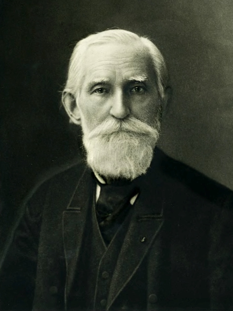
The bound is often called the Bienayme-Chebyshev inequality. Irenee-Jules Bienayme first published it in an 1853 memoir, fourteen years before Pafnuty Chebyshev published his own proof in 1867 (MacTutor History of Mathematics Archive, University of St Andrews).

A few traps come up again and again:
- People often read at least 75 percent as the exact figure, or turn it into a hard count like exactly 75 of my 100 points are inside. It is a floor for any shape; the real number can be anywhere from 75 percent up to 100 percent.
- People often pair the rule with the wrong distribution: using the empirical rule on skewed or unknown data, or reaching for Chebyshev on data they already know is normal and then feeling let down by the loose 75 percent. A simple guide: the empirical rule is for known bell shapes and gives the exact figure; Chebyshev is for any shape and gives the minimum only.
- People often think the tool is broken at k of 1 or below: at k of 1 the bound is 0 percent and below 1 it goes negative, which reads like an error rather than the no-information zone it is. Some also forget that k is the value minus the mean, divided by the standard deviation, and can be a decimal like 1.25.
What this tool does that others don’t
- It derives k correctly from an asymmetric range. When your interval is not centered on the mean, this tool uses the nearer bound, the smaller of the two distances divided by the standard deviation. Tools that assume a symmetric interval read k off the far bound and report a guarantee that is too high. For a mean of 100, a standard deviation of 10, and a range from 70 to 160, this tool gives k of 3, not the over-confident 6.
- It shows the maximum proportion outside k standard deviations, not just the minimum inside. Many calculators return only the within figure. Seeing 1 over k squared next to 1 minus 1 over k squared makes it clear the two parts add up to all of your data.
- It turns the percentage into a guaranteed minimum count for your sample. Enter a sample size n and the tool reports the fewest of your points the bound allows inside, the floor of n times the proportion, so at least 75 of 100 points instead of an abstract 75 percent.
- It puts the Chebyshev floor next to the empirical rule for a normal curve at the same k. The comparison table shows at a glance how conservative the distribution-free bound is, for example 75 percent guaranteed for any shape versus about 95.45 percent for a normal distribution at k of 2.
Limits of this estimate
This calculator gives a guaranteed worst-case floor, not a reading of your own data. Keep these boundaries in mind:
- Chebyshev’s bound is the worst-case floor across every possible distribution, so it understates how much data is actually within k standard deviations for bell-shaped data. It does not give the true proportion for your dataset.
- It cannot tell you the exact percentage of your data within k standard deviations, only a guaranteed minimum. Use it as a distribution-free lower bound, not a measurement of your sample.
- The bound is only meaningful for an effective k greater than 1. At k of 1 or below the formula returns 0 or a negative value, so the calculator requires k greater than 1 in both direct and interval mode.
- Interval mode can only derive k when the standard deviation is positive, the lower bound is below the upper bound, and the mean lies strictly between them. Otherwise, or if the derived k is 1 or less, it shows a status message rather than a bound.
- The guaranteed minimum count is the percentage floor times n rounded down: a deterministic lower limit implied by the bound, not a statistical expected count or a prediction of how many of your points are actually inside k standard deviations.
- It uses the mean and standard deviation you enter and does not compute them from raw data. If those are sample estimates rather than the true population values, the guarantee carries that estimation error.
- In interval mode the effective k uses the smaller of the two distances from the mean to the ends of the range, the nearer bound divided by the standard deviation. For an asymmetric range this is deliberately lower than the naive symmetric k, so the guaranteed proportion can be much smaller than competitor tools report. It is the only bound Chebyshev actually guarantees across the whole interval.
- Percentages are rounded to two decimals and proportions to four, and the within and outside percentages are reported so they sum to exactly 100 percent. A single rounded value can therefore differ from the unrounded figure by up to about 0.005 percentage points.
- The guaranteed minimum count floors the exact, unrounded proportion times n before rounding, so it can be one less than n times the rounded percentage on screen. At k of 3 with 100 points, for example, 88.889 floors to 88, not 89.
Frequently asked questions
What is Chebyshev’s inequality in simple terms?
For any dataset, no matter its shape, at least 1 minus 1 over k squared of the values lie within k standard deviations of the mean. It gives a guaranteed worst-case floor, not the exact percentage.
How do you calculate k in Chebyshev’s theorem?
k is how many standard deviations a value is from the mean: k equals the absolute difference between x and the mean, divided by the standard deviation. If you have an interval around the mean, k equals (b minus mean) over sigma for a symmetric interval, or min(mean minus a, b minus mean) over sigma if the interval is not equidistant from the mean. Switch this tool to interval mode and it does that for you.
Why must k be greater than 1?
At k equals 1 the formula gives 1 minus 1 over 1, which is 0, and at k below 1 it goes negative. The bound only conveys information for k above 1, so the calculator requires the effective k to exceed 1 in both modes.
What does the calculator do if my interval is invalid?
In interval mode the standard deviation must be positive, the lower bound must be below the upper bound, and the mean must lie between them so both distances are positive. If any of those fail, or the derived k comes out at 1 or below, the tool shows a status message instead of a bound rather than a misleading number.
What is the minimum percentage within 2 and 3 standard deviations?
At least 75 percent of any dataset lies within 2 standard deviations (1 minus one quarter), and at least 88.89 percent within 3 standard deviations (1 minus one ninth), regardless of distribution shape.
Is the minimum count an expected value?
No. The guaranteed minimum count is n times (1 minus 1 over k squared) rounded down, a deterministic floor implied by the proportion bound. It is the fewest of your n points that can be inside k standard deviations, not a statistical expectation.
Is Chebyshev’s theorem the same as the empirical rule?
No. The empirical rule (about 68, 95, and 99.7 percent) applies only to roughly normal, bell-shaped data and gives the actual percentages. Chebyshev applies to every distribution but only gives a guaranteed minimum, which is much looser: 75 percent versus about 95 percent at k equals 2.
Does Chebyshev’s inequality apply to all distributions?
Yes, as long as the distribution has a finite mean and standard deviation. That generality is why the bound is conservative compared with shape-specific rules.
Sources
- Chebyshev’s Theorem, Emory University (Oxford College) Math Center, MATH117. States the theorem and the at-least 1 minus 1 over k squared bound for any distribution.
- Chebyshev’s inequality, Wikipedia. Background, the general statement, and the proof from Markov’s inequality.
- Using Chebyshev’s Inequality to Determine Sample Size in Biometric Evaluation of Fingerprint Data, NIST. A real application that leans on the bound when no distribution can be assumed.
- 68-95-99.7 rule, Wikipedia. The empirical-rule percentages for a normal distribution, used here only for the looseness comparison.